How we estimate training runtime and check the forecast
· Denis Voronko
Before loading a model, we want a useful answer to a practical question: how long should this configuration take? Once the job starts, we want to see whether the estimate still makes sense.
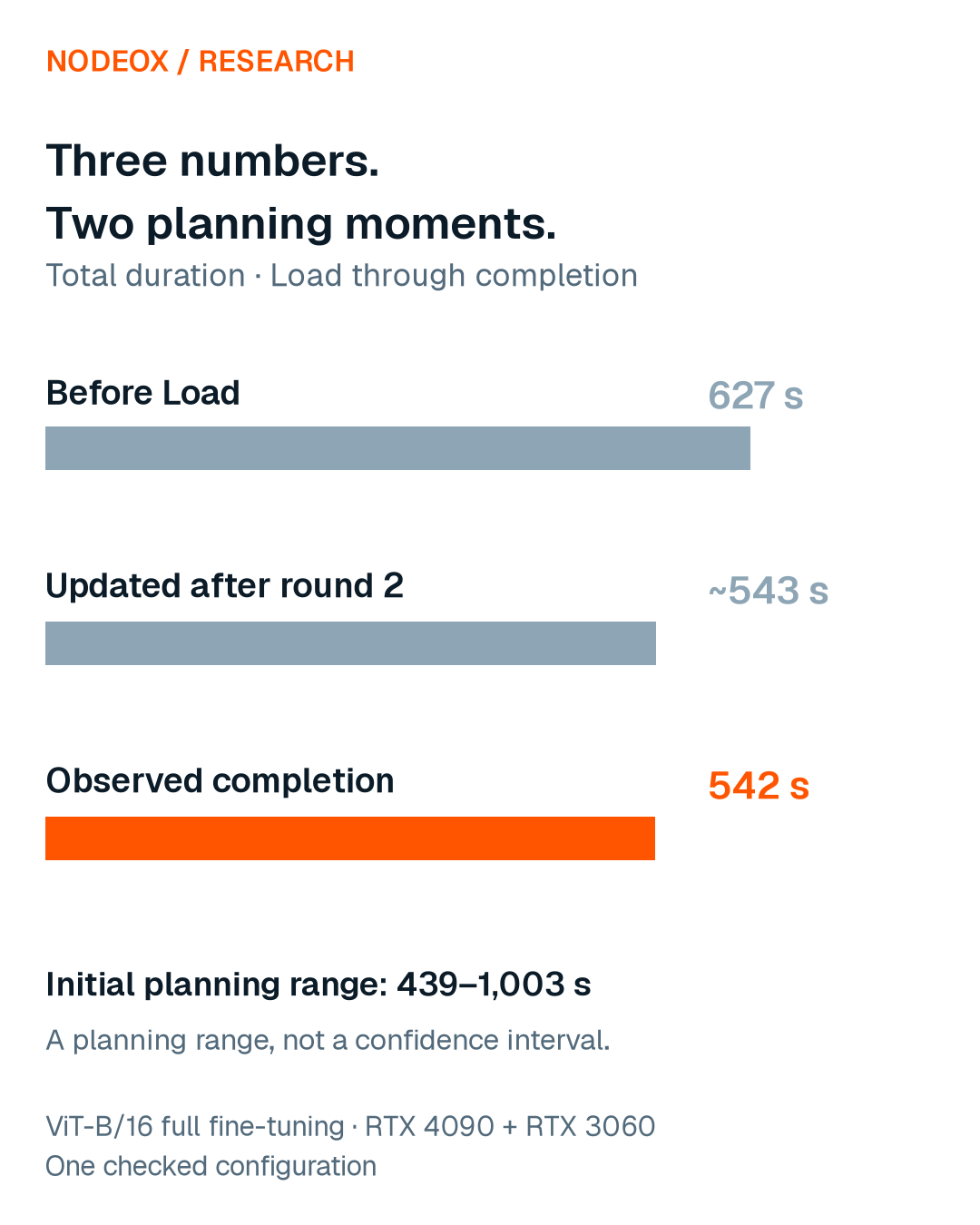
We added that comparison to the Nodeox Workbench. In a full fine-tuning check on an RTX 4090 and RTX 3060, the estimate before Load was 627 seconds. The run took 542 seconds. After round 2, the updated estimate was about 543 seconds. This is how we build, record and check those estimates.
Define what the clock includes
Training time alone does not describe the whole wait in the Workbench. The forecast separates Load, training, exchange and evaluation where configured. Changing the hosts, amount of work or evaluation settings changes the job being estimated.
We keep the estimate made before Load. That preserves the expectation we planned with, even after measurements from the running job become available.
For the live check below, the reported total includes the Load interval and four training rounds. The measured Load interval includes up to ten seconds spent in Ready. Time spent waiting for a user action can therefore affect the comparison.
The distinction between scheduling, orchestration and execution matters here: this forecast covers the run from Load to its result, rather than time waiting in a scheduler’s queue.
Use the information available before the run
Before Load, the Workbench has the selected model and training settings, the candidate hosts’ capabilities, reference speed information and link measurements. Those inputs support an initial estimate and a range.
As our ViT-H coordination memory study shows, fitting the configuration into memory is one prerequisite. The amount of work matters alongside host speed. Batch size, training steps, round count and how the work is split all describe the configuration being timed. A GPU name alone leaves out too much.
Link measurements also deserve inspection. During this session, two rented RTX 4090s measured 52 and 4 Mbit/s download. With both selected, the estimate rose to about 39 minutes, 23 of them for Load, because of the slow link. The automatic selection took one RTX 4090.
The initial range is a planning range. We have not established it as a statistical confidence interval with a measured coverage probability.
Learn from useful measurements in the session
Once a run is in progress, we have information that was unavailable before Load: the hosts’ measured training speeds and the phases already completed.
The Workbench’s session-speed calculation uses training steps divided by training time from round 2 onward, for rounds lasting at least twenty seconds. The warm-up round and very short measurements do not supply the same basis for the next estimate.
The measured speeds can inform the next forecast for the same model and training method. They are drawn from the last run’s timeline, which survives a page reload and is cleared by Reset.
During the current run, the forecast card shows the original estimate and actual progress. From the end of round 2 it also shows an updated total: elapsed time plus an estimate of the remaining work. The displayed remaining-time range narrows as less work is left.
The full fine-tuning check
We checked the deployed forecast on 2 November 2026. The workload was ViT-B/16 from the public library, fine-tuned on Oxford-IIIT Pet, using an NVIDIA RTX 4090 and an NVIDIA RTX 3060. It ran four rounds of 300 training steps split equally across the hosts, with batch size 32.
The estimate before Load was 627 seconds, with a range of 439–1,003 seconds. Completion at 542 seconds fell inside that range. The table separates the initial estimate from the later update.
Quantity | Estimate, seconds | Observed completion, seconds |
|---|---|---|
Total before Load | 627 (439–1,003) | 542 |
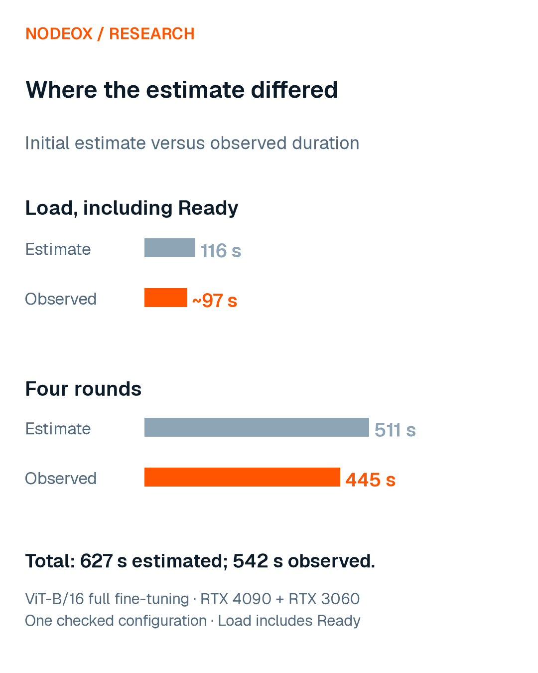
Load, including Ready | 116 | About 97 |
Four rounds | 511 | 445 |
Updated total after round 2 | About 543 | 542 |
Read the difference correctly
The run finished 85 seconds sooner than the initial estimate: about 13.6% below it. That is the deviation between a prediction and the completed run.
Part of the gap is in how the estimate treats a round: it adds the exchange after the training. In the run, the RTX 4090 finished its half of the steps well before the RTX 3060 and sent its update while the 3060 was still training. As our E1 study found, hosts work in parallel, so their phases cannot simply be added. The speeds measured in the session, 2.2 and 0.46 times an NVIDIA A40, matched our reference table, so the speed inputs were right. Actual round durations were 130, 105, 108 and 102 seconds.
The updated estimate after round 2 was close to the final duration because it could use information from the job already in progress. The approximately 543 seconds meant the expected total duration, not another 543 seconds still to wait.
These are different planning moments. The estimate before Load helps us choose and prepare a configuration; the later estimate helps us understand the run we have already started.
Keep the original forecast in the record
A forecast is easier to evaluate when it remains beside the result. At Load, the Workbench sends the estimate and its inputs; the coordinating process validates and records them as a run event.
The timeline then carries the original estimate, observed progress and update. A reloaded page and a shared-run viewer can display the same run-level comparison. A completed run shows its elapsed time and deviation from the estimate before Load.
Keeping this record avoids evaluating the initial estimate against a number that has already been replaced by a later prediction. It also gives the next engineering check a concrete question: which phase explained the difference?
What this check establishes
For this full fine-tuning configuration, the completed run landed inside the initial planning range, and the estimate updated from in-run measurements was close to the finish time.
A single checked configuration does not establish forecast accuracy across model families, host combinations or networks. The way to extend the evidence is to retain original estimates and compare them with completed runs under stated conditions.
Result quality is checked separately. A useful time estimate helps plan the run; an evaluation tells us whether its output is acceptable.
From a number to a usable comparison
The improvement is that the estimate now has a visible life cycle: an expectation before Load, measured progress during training, and a result we can inspect afterwards.
We can choose a candidate configuration with that expectation in view, update our understanding as the run proceeds, and keep the comparison for the next test. That is the standard we want the forecast to meet.