How we brought ViT-H coordination below a 16 GB memory budget

November 8, 2026 · Denis Voronko

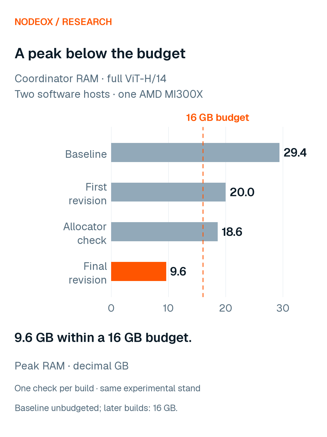
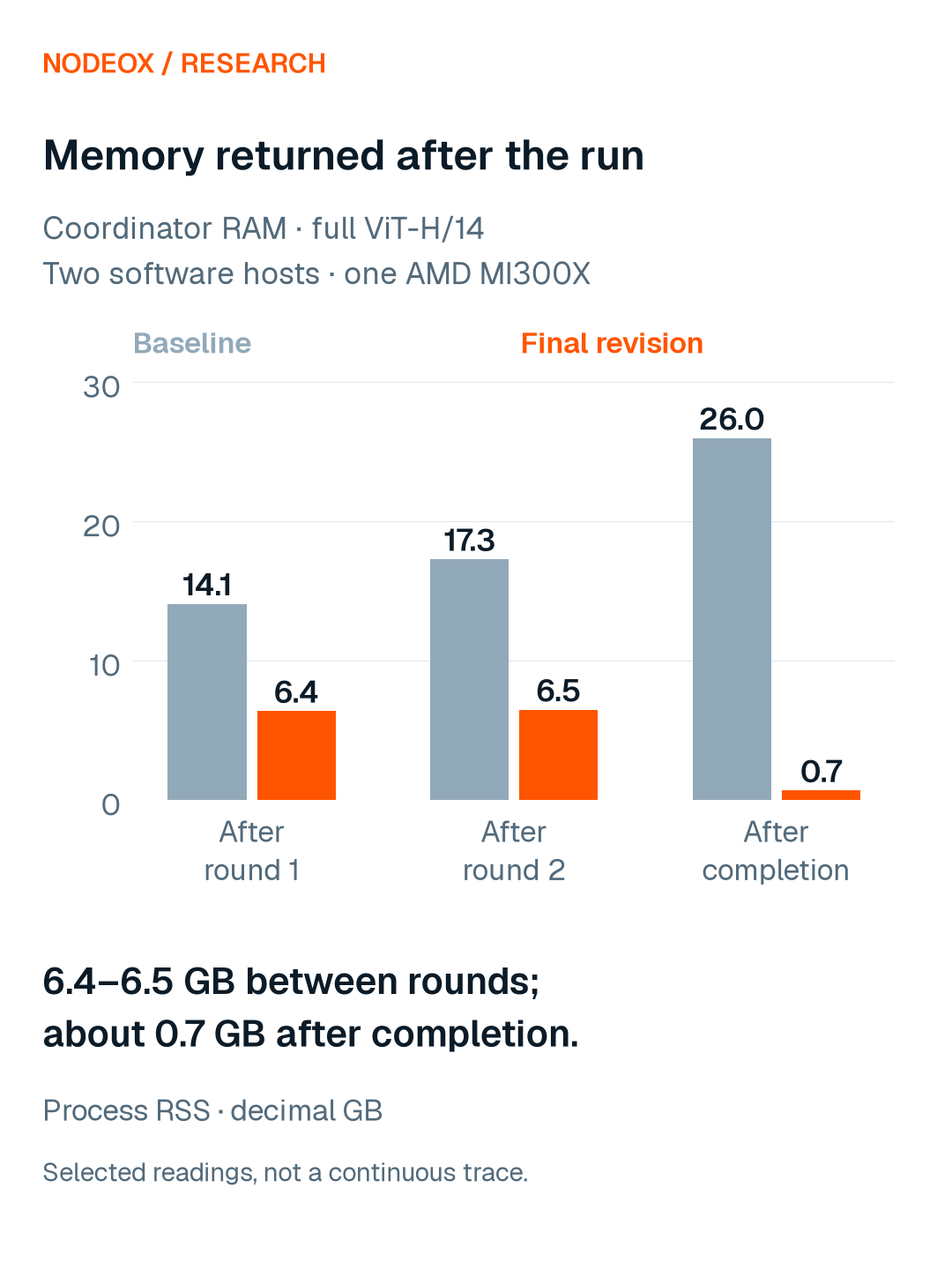
A full ViT-H/14 run used almost 30 GB of RAM in our coordinating process. After changing how model state was held, saved and released, the same engineering check peaked at 9.6 GB. Between rounds, memory stayed level; after the run, RSS returned to about 0.7 GB.

The interesting part was finding what remained alive. Reducing temporary copies helped, but a reference cycle in the aggregation code kept two full model states around each round. Our test helper’s own garbage collection had hidden it. A live run made the remaining problem visible.

This follows our E1 study of distributed training overhead, which traced time and memory costs outside GPU computation.

The question: where did the model-sized copies go?

The model’s fp32 weights were roughly 2.5 GB. Coordinating training also required persistent working state and temporary buffers, whose memory use changed across phases.

Those objects have different lifetimes. Some must survive between rounds. Others should become unreachable as soon as a phase ends. We wanted to bring the coordinating process within a 16 GB memory budget and release its working memory when the run finished.

This was a process-RAM investigation. The GPU’s available memory and the model’s training-memory requirement were separate constraints.

Experimental setup

We checked full fine-tuning of ViT-H/14 on one AMD MI300X cloud instance, with two software GPU hosts sharing that card. Each run used three rounds, batch size 32 and 20 training steps per host per round.

The coordinating stand ran successive engineering builds. The baseline preceded the memory changes. Later runs tested the first revision, an allocator-setting variant, and the final revision with the aggregation namespace cleared. The model and training settings were held constant across the builds.

The baseline’s memory was sampled from the process every two seconds. Later builds also recorded memory events around Load, aggregation, synchronization and saving. We compared the process peak, RSS between rounds and RSS after completion. Values below use decimal GB.

What the successive runs showed

The first revision brought the peak down, but the live trace still climbed between rounds. That was useful evidence: lowering the largest temporary allocation had not explained everything.

The final revision met the budget and removed that growth. The table keeps the intermediate attempts because they show how we reached the result.

Reduce copies and keep less state resident

We reduced the number of full-size copies, moved state that can wait out of RAM, and made the memory budget an explicit admission check.

At completion, working state was released after the run’s outstanding work returned. The budget and admission checks also became explicit: a Load estimated not to fit was refused before taking GPU hosts. For this run, the estimate was 11.1 GB, above the 9.6 GB it used.

These changes formed a package. The overall reduction from the baseline to the final run cannot be attributed to the last namespace fix alone.

The cycle we found live

The aggregation template defines functions. A Python function retains its global namespace; in this case, that namespace also held references to the original and resulting model states.

That created a cycle. The model objects could stay alive after their phase had finished, until cyclic garbage collection ran. In the live checks, the first revision retained roughly two more full-size models per round.

The unit-test copy counter called garbage collection itself. That made its measurements useful for counting copies, but it also removed the cycle before the test observed the live behavior.

We cleared the aggregation execution namespace once its work was finished and added a test with cyclic collection disabled. The new test exercised the lifetime problem instead of cleaning it up first. In the final live run, between-round RSS stayed at about 6.4–6.5 GB.

Check the time cost as well

Reducing the resident working set introduced additional I/O, costing about 1.6 seconds per round in this check.

We also tracked the interval from aggregation completing to synchronization starting. In the final run, the two measured intervals were 6.75 and 5.00 seconds, against 5.28 and 3.48 seconds in the baseline, below the ten-second acceptance target used in the session. This interval is one phase boundary, rather than the duration of an entire training round.

The memory result therefore came with an observed time trade-off: about 1.5 seconds per round at one phase boundary, for about 20 GB less at the peak. How we benchmark mixed-GPU training explains why we time each phase separately.

What we verified

The final run’s recorded peak was 9,642,319,872 bytes, or 9.642 GB. It stayed within the imposed 16 GB budget, between-round RSS was level, and the post-run reading was about 0.7 GB.

The run completed all six host updates and all four between-round host synchronizations without a full-model fallback. These checks cover the execution path exercised by this run; training-result quality requires its own evaluation.

The recorded experiment used one run of each engineering configuration on two software hosts sharing one card. It establishes the result for that setup; a larger physical fleet is a separate check.

What we took from it

The useful change was making state lifetime inspectable. A model-size calculation told us what one copy cost. Phase-level memory readings showed how many copies survived and when the working set should fall.

The final configuration brought a full ViT-H coordination run within its budget and returned memory afterwards. It also left us with a better test: one that could expose the lifetime problem without collecting it away first.